NOTE: The figures in this section are relatively small in order to allow them to be displayed quickly. The "Fig. N" link beneath each figure points to a PDF version of the figure. These are in vector format and allow the figures to be magnified to show the details more clearly.
The primary sources for the material presented here are:
- J. P. Snyder, Map Projections: A Working Manual, USGS Professional Paper 1395 (1987), pp. 48–66. This contains an overview of the transverse Mercator projection (and many other projections). However, the approximations given for this projection are rather crude. The terminology for the various transverse Mercator map projections is taken form J. P. Snyder, Flattening the Earth (Chicago Univ. Press, 1993).
- L. Krüger, Konforme Abbildung des Erdellipsoids in der Ebene (Conformal mapping of the ellipsoidal earth to the plane), Royal Prussian Geodetic Institute, New Series 52, 172 pp. (1912). The derives the series solution for the transverse Mercator projection of an ellipsoid. This gives very good accuracy and this method or an extension of it to higher-order provides the most accurate algorithms for the projection valid in some zone near the central meridian. It is also of interest to see the systematic use of logarithms in the pre-electronic and pre-mechanical age (when computers were human).
- JHS 154, ETRS89 - järjestelmään liittyvät karttaprojektiot, tasokoordinaatistot ja karttalehtijako (Map projections, plane coordinates, and map sheet index for ETRS89), published by JUHTA, Finnish Geodetic Institute, and the National Land Survey of Finland (2006). A concise summary of Krüger's method is given in Appendix 1.
- L. P. Lee, Conformal Projections Based on Elliptic Functions, (B. V. Gutsell, Toronto, 1976), 128pp., ISBN: 0919870163 (Also appeared as: Monograph 16, Suppl. No. 1 to Canadian Cartographer, Vol 13). Part V, pp. 67–101, Conformal Projections Based On Jacobian Elliptic Functions, gives closed form expressions for the transverse Mercator projection based on work by Thompson (1945). This may be purchased for a modest sum. Other useful sections are Part I, pp. 1–3 and Part II, pp. 4–14.
- M. Abramowitz and I. A. Stegun, Handbook of Mathematical Functions (Dover, 1965). This is the bible for special functions. It is easily accessible on the web. Chapter 16 covers elliptic functions and Chapter 17 covers elliptic integrals.
Survey of transverse Mercator projections
The following is adapted from Lee (1976) particularly pp. 92–101. The terminology is from Snyder (1993) pp. 159–161.
The transverse Mercator projection is a conformal projection of the ellipsoid in which the central meridian is straight. Within these constrains there are various projections that differ in how the scale varies along the central meridian. The simplest such projection from an algorithmic point of view is the Gauss-Schreiber projection which consists of a conformal projection from the ellipsoid to a sphere followed by the spherical transverse Mercator projection. This results in a projection whose scale on the central meridian increases from the equator to the pole (by an amount proportional to the flattening). In the Gauss-Krüger projection, the scale along the central meridian is held constant. This projection is usually expressed as a series which is valid only sufficiently close to the central meridian. (This is implemented by GeographicLib::TransverseMercator.) The projection can however be expressed in closed form in terms of the Thompson transverse Mercator projection (where the scale along the central meridian decreases from the equator to the pole by an amount proportional to the flattening). (This method of computing the Gauss-Krüger projection is implemented by GeographicLib::TransverseMercatorExact.)
The graticules (lines of constant latitude and longitude) for all these projections are shown in Figs. 1–3. These figures all use an ellipsoid with eccentricity e = 1/10 (inverse flattening = 10 (3 sqrt(11) + 10) = 199.5, i.e., somewhat flatter than the WGS84 ellipsoid) and the projections have all been scaled so that the distance from the equator to the north pole is unity. One eighth of the ellipsoid is shown in these figures, 0o <= latitude <= 90o and 0o <= longitude <= 90o. To obtain the graticule for the entire ellipsoid reflect these figures in x = 0, y = 0, and y = 1. The blue lines show latitude and longitude at multiples of 10o. The green lines show 1o intervals for longitude in [80, 90] and latitude in [0, 10]. In all three figures, longitude = 0o lies on x = 0 and longitude = 90o lies on y = 1.
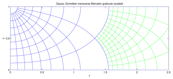
The graticule for the Gauss-Schreiber transverse Mercator projection. The equator lies on y = 0. Compare this with Lee, Fig. 1 (right), which shows the graticule for half a sphere, but note that in his notation x and y have switched meanings. The graticule for the ellipsoid differs from that for a sphere only in that the latitude lines have shifted slightly. (The conformal transformation from an ellipsoid to a sphere merely relabels the lines of latitude.) This projection places the point latitude = 0o, longitude = 90o at infinity.
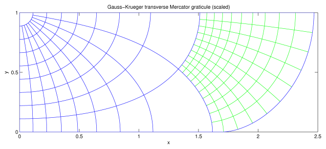
The graticule for the Gauss-Krüger transverse Mercator projection. The equator lies on y = 0 for longitude < 81o; beyond this, it arcs up to meet y = 1. Compare this with Lee, Fig. 45 (upper), which shows the graticule for the International Spheroid. Lee, Fig. 46, shows the graticule for the entire ellipsoid. This projection (like the Thompson projection) projects the ellipsoid to a finite area.
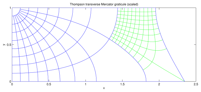
The graticule for the Thompson transverse Mercator projection. The equator lies on y = 0 for longitude < 81o; at longitude = 81o, it turns by 120o and heads for y = 1. Compare this with Lee, Fig. 43, which shows the graticule for the International Spheroid. Lee, Fig. 44, shows the graticule for the entire ellipsoid. This projection (like the Gauss-Krüger projection) projects the ellipsoid to a finite area.
Of the three transverse Mercator projections given here the Gauss-Krüger projection is by far the most important. It is the basis of the UTM system. If "transverse Mercator projection" is used without further elaboration, then, nearly always, it refers to the Gauss-Krüger projection.
Properties far from the central meridian
The divergent behavior of the Gauss-Schreiber projection as latitude = 0o, longitude = 90o is approached is unsurprising given the behavior of the standard Mercator projection at the poles. On the other hand, the lack of divergence in the Gauss-Krüger projection (and similarly in the Thompson projection) is perhaps puzzling. We explore the behavior more carefully in this section.
Firstly, the Gauss-Krüger projection does have a singularity at latitude = 0o and longitude < 90o(1 - e), where e is the eccentricity of the ellipsoid. The choice of e = 1/10 for Figs. 1–3 was made to ensure that one of the graticule lines (longitude = 81o) covered this singularly. The singularly is relatively benign. The Thompson projection contains a cube root singularity with causes the corner in the equator. The transformation from Thompson to Gauss-Krüger "repairs" this to lowest order so that there's no kink in the equation. Nevertheless, a weaker singularity remains (causing a discontinuous change in the radius of curvature for the equator). Thus Gauss-Krüger has a branch point at latitude = 0o and longitude < 90o(1 - e) and the projection is analytic provided this point is avoided. However the results obtained for the projection will depend on which sheet of the projection is used or which route around the branch point is taken.
The "standard" convention for projecting a geographic position is to follow the central meridian from the equator to the target latitude, then to follow the line of constant latitude to the target longitude. This is equivalent to placing two branch cuts on the equator in the longitude ranges +/- [90o(1 - e), 90o(1 + e)]. For points on equator for |longitude| > 90o(1 - e), the path should go to the north of branch point. This convention corresponds to Fig. 2, above, after suitable reflections to cover the ellipsoid and to Lee, Fig. 46.
In order to explore the behavior to the right of the equator in Fig. 2, we define an "extended" domain for the projection, this consists of the union of
- 0o <= latitude <= 90o and 0o <= longitude <= 90o
- -90o < latitude <= 0o and 90o(1 - e) <= longitude <= 90o
The rule for reaching the second area here is to move on the central meridian to a small positive latitude, move at constant latitude to the target longitude and then to move on a meridian to the target latitude. In this case, the branch cut emanates in a south-westerly direction from the branch point. Following this prescription the range of the projection now consists of the union of
- 0 <= x and 0 <= y/(k0 a) <= E(e2)
- K(1 - e2) - E(1 - e2) <= x/(k0 a) and y <= 0
where k0 is the central scale factor, a is the major radius of the ellipsoid, K and E are complete elliptic integrals. Setting the optional argument extendp = true in the constructor for GeographicLib::TransverseMercatorExact provides access to this extended domain.
Figures 4–5 illustrate the properties of the Gauss-Krüger transverse Mercator projection in this extended domain. These figures use an ellipsoid with eccentricity 1/10 (as in Figs. 1–3) and with a = 1/E(0.01) = 0.6382 and k0 = 1. The branch point in this case lies at lat = 0o, lon = 81o or x = (K(0.99) - E(0.99))/E(0.01) = 1.71, y = 0.
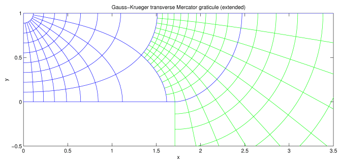
Figure 4 shows the graticule the extended domain. The blue lines show latitude and longitude at multiples of 10o. The green lines show 1o intervals for longitude in [80, 90] and latitude in [-5, 10].
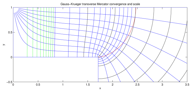
Figure 5 shows the convergence and scale for the Gauss-Krüger transverse Mercator projection in the extended domain. The blue lines emanating from the top left corner (the north pole) are lines of constant convergence. Convergence = 0o is given by the dog-legged line joining the points (0,1), (0,0), (1.71,0), (1.71,-inf). Convergence = 90o is given by the line y = 1. The other lines show multiples of 10o between 0o and 90o. The other blue, the green and the black lines show scale = 1 thru 2 at intervals of 0.1, 2 thru 15 at intervals of 1, and 15 thru 35 at intervals of 5. Multiples of 5 are shown in black, multiples of 1 are shown in blue, and the rest are shown in green. Scale = 1 is given by the line segment (0,0) to (0,1). The red line shows the equator between lon = 81o and 90o. The scale and convergence at the branch point are 1/e = 10 and 0o, respectively.
Symmetries in the projection can now be employed to extend the Gauss-Krüger transverse Mercator projection with arbitrary rules for how to circumvent the branch point. The symmetries are equivalent to placing mirrors on the lines segments
- 0 <= x, y = 1
- x = 0, 0 <= y <= 1
- 0 <= x <= 1.71, y = 0
- x = 1.71, y <= 0
In order to understand the projection better, it is instructive to examine the Thompson projection in the extended domain.
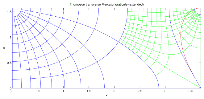
Figure 6 shows the graticule for the Thompson transverse Mercator projection for the extended domain. The range of the projection is the rectangular region shown
- 0 <= u <= K(e2), 0 <= v <= K(1 - e2)
The coloring of the lines is the same as Fig. 4, except that latitude lines extended down to -10o and a red line has been added showing the line y = 0 for x > 1.71 in the Gauss-Krüger projection (Fig. 4). The extended Thompson projection figure has reflection symmetry on all the four sides of Fig. 6.
In transforming from Thompson to Gauss-Krüger, the right angle at lower right corner of Fig. 6 expands by 3 to 270o to produce the outside corner at x = 1.71 and y = 0 in Fig. 4. The top right corner of Fig. 6 represents the south pole and this is transformed to infinity in the extended Gauss-Krüger projection. Despite the apparent similarities, the behavior of north and south poles in the extended Thompson projection (top left and top right corners in Fig. 6) is rather different. The singularity for the north pole is merely the result of the singularity of a polar coordinate system (e.g., longitude is undefined at the north pole). Encircling the north pole, causes longitude to increase by 360o, as expected. On the other hand, encircling the south pole in increasing the longitude by 360o e = 36o. The same behavior is exhibited by the extended Gauss-Krüger projection. The point latitude = -1o, longitude = 90o projects to a point [2.65,1] in Fig. 4. If we now travel along this latitude line to longitude = 54o = 90o - 36o we arrive back at the same projected position. In the extended domain, the Thompson and the Gauss-Krüger projections are not tightly tied to the globe but can slip around it longitudinally.
Test data for the transverse Mercator projection
A test set for the transverse Mercator projection is available at
This is about 17 MB (compressed). This test set consists of a set of geographic coordinates together with the corresponding transverse Mercator coordinates. The WGS84 ellipsoid is used, with central meridian 0o, central scale factor 0.9996 (the UTM value), false easting = false northing = 0 m.
Each line of the test set gives 6 space delimited numbers
- latitude (degrees, exact)
- longitude (degrees, exact — see below)
- easting (meters, accurate to 0.1 pm)
- northing (meters, accurate to 0.1 pm)
- meridian convergence (degrees, accurate to 10-18 deg)
- scale (accurate to 10-20)
The latitude and longitude are all multiples of 10-12 deg and should be regarded as exact, except that longitude = 82.63627282416406551 should be interpreted as exactly 90 (1 - e) degrees. These results are computed using Lee's formulas with Maxima's bfloats and fpprec set to 80 (so the errors in the data are probably 1/2 of the values quoted above). The Maxima code, tm.mac and ellint.mac, used to prepare this data set is included in the distribution. You will need to have Maxima installed to use this code. The comments at the top of tm.mac illustrate how to run it.
The contents of the file are as follows:
- 250000 entries randomly distributed in lat in [0, 90], lon in [0, 90];
- 1000 entries randomly distributed on lat in [0, 90], lon = 0;
- 1000 entries randomly distributed on lat = 0, lon in [0, 90];
- 1000 entries randomly distributed on lat in [0, 90], lon = 90;
- 1000 entries close to lat = 90 with lon in [0, 90];
- 1000 entries close to lat = 0, lon = 0 with lat >= 0, lon >= 0;
- 1000 entries close to lat = 0, lon = 90 with lat >= 0, lon <= 90;
- 2000 entries close to lat = 0, lon = 90 (1 - e) with lat >= 0;
- 25000 entries randomly distributed in lat in [-89, 0], lon in [90 (1 - e), 90];
- 1000 entries randomly distributed on lat in [-89, 0], lon = 90;
- 1000 entries randomly distributed on lat in [-89, 0], lon = 90 (1 - e);
- 1000 entries close to lat = 0, lon = 90 (lat < 0, lon <= 90);
- 1000 entries close to lat = 0, lon = 90 (1 - e) (lat < 0, lon <= 90 (1 - e));
(a total of 287000 entries). The entries for lat < 0o and lon in [90o (1 - e), 90o] use the "extended" domain for the transverse Mercator projection explained in Properties far from the central meridian. The first 258000 entries have lat >= 0o and are suitable for testing implementations following the standard convention.
The errors in the forward and reverse projections are converted into a ground distance (e.g., by dividing the error in the projection by the scale factor). The errors in the convergence and in the scale may be large because these quantities vary rapidly near singular points (for convergence at the lat = 90o and for both convergence and scale at lat = 0o, lon = 90o (1 - e)). We account for this by expressing the error as the sum of a constant and a term proportional to the gradient of the quantity being measured.
Accuracy of transverse Mercator projection
Errors in GeographicLib::TransverseMercatorExact. For both Forward and Reverse projections
- error in position < 8 nm
- error in convergence, d(gamma) < 2e-15" + 8 nm . grad(gamma)
- relative error in scale, dk/k < 7e-12%% + 3 nm . grad(k)/k
These errors apply with the standard convention for the transverse Mercator projection. In this case, we use only test samples with non-negative values of latitude.
For the extended transverse Mercator projection (Fig. 4), the errors given above apply only for latitude >= -15o. For more negative latitudes, the errors become large. For example for latitude >= -58o, the maximum error is 1 mm (and the scale has become 124 million). This increase in the error is due to the use of the Thompson projection in the computation. Looking at the graticule for this projection (Fig. 6), we see that the Thompson scale becomes small close to the south pole resulting in errors (measured as a ground distance) which diverges (the errors vary inversely with scale). For example at lat = -58o, the scale for the Thompson projection is about 240000 times smaller than on the central meridian and the errors have increased by about the same factor. If necessary, this problem could be avoided by reformulating the Thompson projection to place the origin at the South pole.
If GeographicLib::TransverseMercatorExact is modified to use long doubles (a 64-bit floating fraction) instead of of doubles (53-bit floating fraction) then the error in the position is about 4 pm, for latitude >= -15o.
Errors in GeographicLib::TransverseMercator. For both Forward and Reverse projections with easting |x| <= 4200 km (approximately within 35o of the central meridian) using the 6th-order series (TM_TX_MAXPOW = 6, the default)
- error in position < 5 nm
- error in convergence, d(gamma) < 7e-10" + 5 nm . grad(gamma)
- relative error in scale, dk/k < 6e-12%%
The error in the scale does not need to include a grad(k) term because the scale varies smoothly within this region. If instead we restrict |x| <= 3400 km (approximately within 29o of the central meridian), we get a tighter bound on the convergence
- error in convergence, d(gamma) < 2e-15" + 5 nm . grad(gamma)
Further from the central meridian, the errors grow rapidly. For |x| = 10700 km (approx 68o from the central median), the error in position is about 1 mm. When used in the UTM system, x is typically restricted to |x| <= 500 km. Within |x| <= 500 km, the errors using the 6th-order series are dominated by round-off rather than the number of terms. If GeographicLib::TransverseMercator is modified to use long double instead of double, the error in the position within the the UTM region is about 4 pm.
If GeographicLib::TransverseMercator is compiled with TM_TX_MAXPOW = 4 to give the 4th-order approximation, then the error is about 210 nm for |x| <= 500 km (the region used for UTM coordinates).
Series approximation for transverse Mercator
Krüger (1912) gives a 4th-order approximation to the transverse Mercator projection. The method entails performing first a Gauss-Schreiber projection and approximating the warp of this to Gauss-Krüger projection as a series in n = (a - b)/(a + b). This is accurate to about 200 nm within the UTM domain. Here we present the series extended to 12th order. We follow the notation of JHS 154.
By default, GeographicLib::TransverseMercator uses the 6th-order approximation. The preprocessor variable TM_TX_MAXPOW can be used to select an order from 4 thru 8.
In the formulas below ^ indicates exponentiation (n^3 = n*n*n) and / indicates real division (3/5 = 0.6). The equations need to be converted to Horner form, but are here left in expanded form so that they can be easily truncated to lower order in n. Some of the integers here are not representable as 32-bit integers and will need to be included as double literals.
Eq. (01) [A in Krüger, p. 12, eq. (5)]
  A1 = a/(n + 1) * (1 + 1/4 * n^2
                      + 1/64 * n^4
                      + 1/256 * n^6
                      + 25/16384 * n^8
                      + 49/65536 * n^10
                      + 441/1048576 * n^12);
Eqs. (06) [beta in Krüger, p. 18, eq. (26*)]
  h[1]   =   1/2 * n
           - 2/3 * n^2
           + 37/96 * n^3
           - 1/360 * n^4
           - 81/512 * n^5
           + 96199/604800 * n^6
           - 5406467/38707200 * n^7
           + 7944359/67737600 * n^8
           - 7378753979/97542144000 * n^9
           + 25123531261/804722688000 * n^10
           - 9280258847/6437781504000 * n^11
           - 1628053924171/99584432640000 * n^12;
  h[2]   =   1/48 * n^2
           + 1/15 * n^3
           - 437/1440 * n^4
           + 46/105 * n^5
           - 1118711/3870720 * n^6
           + 51841/1209600 * n^7
           + 24749483/348364800 * n^8
           - 115295683/1397088000 * n^9
           + 5487737251099/51502252032000 * n^10
           - 5845886411021/41845579776000 * n^11
           + 6339155669701909/46867049349120000 * n^12;
  h[3]   =   17/480 * n^3
           - 37/840 * n^4
           - 209/4480 * n^5
           + 5569/90720 * n^6
           + 9261899/58060800 * n^7
           - 6457463/17740800 * n^8
           + 2473691167/9289728000 * n^9
           - 852549456029/20922789888000 * n^10
           - 2673218294321/191294078976000 * n^11
           - 1619588070701683/35150287011840000 * n^12;
  h[4]   =   4397/161280 * n^4
           - 11/504 * n^5
           - 830251/7257600 * n^6
           + 466511/2494800 * n^7
           + 324154477/7664025600 * n^8
           - 937932223/3891888000 * n^9
           - 89112264211/5230697472000 * n^10
           + 12003335387/32691859200 * n^11
           - 537877266968267441/2249618368757760000 * n^12;
  h[5]   =   4583/161280 * n^5
           - 108847/3991680 * n^6
           - 8005831/63866880 * n^7
           + 22894433/124540416 * n^8
           + 112731569449/557941063680 * n^9
           - 5391039814733/10461394944000 * n^10
           + 4863559943251/167382319104000 * n^11
           + 37588208648677/67596705792000 * n^12;
  h[6]   =   20648693/638668800 * n^6
           - 16363163/518918400 * n^7
           - 2204645983/12915302400 * n^8
           + 4543317553/18162144000 * n^9
           + 54894890298749/167382319104000 * n^10
           - 132058444054073/177843714048000 * n^11
           - 21678380925301381/85364982743040000 * n^12;
  h[7]   =   219941297/5535129600 * n^7
           - 497323811/12454041600 * n^8
           - 79431132943/332107776000 * n^9
           + 4346429528407/12703122432000 * n^10
           + 947319776978297/1625999671296000 * n^11
           - 139564766909992667/115852476579840000 * n^12;
  h[8]   =   191773887257/3719607091200 * n^8
           - 17822319343/336825216000 * n^9
           - 497155444501631/1422749712384000 * n^10
           + 4081516004323/8281937664000 * n^11
           + 3016420810780677019/2994340933140480000 * n^12;
  h[9]   =   11025641854267/158083301376000 * n^9
           - 492293158444691/6758061133824000 * n^10
           - 3340781295639871/6360528125952000 * n^11
           + 230755947172792843/315376186245120000 * n^12;
  h[10]  =   7028504530429621/72085985427456000 * n^10
           - 1396721719354981/13516122267648000 * n^11
           - 242069739433316973869/299733527407362048000 * n^12;
  h[11]  =   20180430688893997/144171970854912000 * n^11
           - 39227670225311092139/261131482210959360000 * n^12;
  h[12]  =   170866240186706518133/831839653739888640000 * n^12;
Eqs. (07) [gamma in Krüger, p. 21, eq. (41)]
  h'[1]  =   1/2 * n
           - 2/3 * n^2
           + 5/16 * n^3
           + 41/180 * n^4
           - 127/288 * n^5
           + 7891/37800 * n^6
           + 72161/387072 * n^7
           - 18975107/50803200 * n^8
           + 60193001/290304000 * n^9
           + 134592031/1026432000 * n^10
           - 1043934033787/3218890752000 * n^11
           + 1107802529272207/5178390497280000 * n^12;
  h'[2]  =   13/48 * n^2
           - 3/5 * n^3
           + 557/1440 * n^4
           + 281/630 * n^5
           - 1983433/1935360 * n^6
           + 13769/28800 * n^7
           + 148003883/174182400 * n^8
           - 705286231/465696000 * n^9
           + 1703267974087/3218890752000 * n^10
           + 490493610499/373621248000 * n^11
           - 1975809888712343/976396861440000 * n^12;
  h'[3]  =   61/240 * n^3
           - 103/140 * n^4
           + 15061/26880 * n^5
           + 167603/181440 * n^6
           - 67102379/29030400 * n^7
           + 79682431/79833600 * n^8
           + 6304945039/2128896000 * n^9
           - 6601904925257/1307674368000 * n^10
           + 35472608886503/41845579776000 * n^11
           + 7660808256523559/1098446469120000 * n^12;
  h'[4]  =   49561/161280 * n^4
           - 179/168 * n^5
           + 6601661/7257600 * n^6
           + 97445/49896 * n^7
           - 40176129013/7664025600 * n^8
           + 138471097/66528000 * n^9
           + 48087451385201/5230697472000 * n^10
           - 634613396309/40864824000 * n^11
           + 152161926556090753/1124809184378880000 * n^12;
  h'[5]  =   34729/80640 * n^5
           - 3418889/1995840 * n^6
           + 14644087/9123840 * n^7
           + 2605413599/622702080 * n^8
           - 31015475399/2583060480 * n^9
           + 5820486440369/1307674368000 * n^10
           + 98568244458947/3678732288000 * n^11
           - 1367520624030470251/29877743960064000 * n^12;
  h'[6]  =   212378941/319334400 * n^6
           - 30705481/10378368 * n^7
           + 175214326799/58118860800 * n^8
           + 870492877/96096000 * n^9
           - 1328004581729009/47823519744000 * n^10
           + 3512873113922087/355687428096000 * n^11
           + 986615629722639449/13133074268160000 * n^12;
  h'[7]  =   1522256789/1383782400 * n^7
           - 16759934899/3113510400 * n^8
           + 1315149374443/221405184000 * n^9
           + 71809987837451/3629463552000 * n^10
           - 52653013293696143/812999835648000 * n^11
           + 101784256296129577/4455864483840000 * n^12;
  h'[8]  =   1424729850961/743921418240 * n^8
           - 256783708069/25204608000 * n^9
           + 2468749292989891/203249958912000 * n^10
           + 117880637749661/2707556544000 * n^11
           - 5921832934345276446697/38926432130826240000 * n^12;
  h'[9]  =   21091646195357/6080126976000 * n^9
           - 67196182138355857/3379030566912000 * n^10
           + 395018924202597949/15446996877312000 * n^11
           + 91220875613845291081/946128558735360000 * n^12;
  h'[10] =   77911515623232821/12014330904576000 * n^10
           - 268897530802721453/6758061133824000 * n^11
           + 8257746726303249815683/149866763703681024000 * n^12;
  h'[11] =   12809767642647461/1029799791820800 * n^11
           - 5303630969873795374429/65282870552739840000 * n^12;
  h'[12] =   2240624428311897034834681/91918281738257694720000 * n^12;
Eqs. (15), (16), (17), (18), (23), (24), (25), (26) of JHS 154 are extended in the obvious way.
The formulas for meridian convergence (34) and scale (35) are only good for small lam (l in the notation of JHS 154). More accurate expressions are given here where ep2 = e'2 = e2/(1 - e2) (eq. 04).
  double
    c = cos(phi),
    s = sin(lam),
    c2 = c * c,
    s2 = s * s,
    d = 1 - s2 * c2,
    // Accurate to order ep2^2
    carg = 1 + c2 * c2 * s2 / d * ep2 *
    (1 + c2 / (3 * d * d) *
     (2 - s2 * (c2 * ((4 * c2 - 1) * s2 - 9) + 8)) * ep2),
    // Accurate to order ep2
    cabs = 1 + c2 * c2 * s2 * ((c2 - 2) * s2 + 1) / (2 * d * d) * ep2;
  // This replaces (34)
  gamma = atan2(sin(phi) * s * carg, cos(lam));
  // This replaces (35)
  k = cabs/sqrt(d);
Unfortunately, expansions of this type are much more messy at higher order. Therefore, For greater accuracy, directly differentiate the series involving h' or h. The accumulation of the sum can be carried out at the same time as the transformation itself (and the calculation slots into a Clenshaw summation very easily). The derivatives give the convergence, gamma'', and scale, k'', of the [xi, eta] (Gauss-Krüger) projection relative to [xi', eta'] (Gauss-Schreiber) projection and vice versa. For the full convergence and scale these need to be compounded with the convergence, gamma', and scale, k', of the Gauss-Schreiber projection.
   gamma = gamma' + gamma''
       k = k' * k''
gamma' and k' are conveniently expressed as
  gamma' = atan(tan(lam) * sin(beta))
         = atan(tan(lam) * tanh(Q))
         = atan(tan(xi') * tanh(eta'))
      k' = sqrt(1 - e^2 * sin(phi)^2)
           * (cos(beta) / cos(phi)) * cosh(eta')
where the factors on the last line are can be computed accurately with
 (cos(beta) / cos(phi)) * cosh(eta')
         = cosh(Q') / hypot(sinh(Q), cos(lam))
         = cosh(Q') * hypot(sinh(eta'), cos(xi'))
These last two expressions preserve accuracy near the pole. See also Krüger, pp. 19–20, eqs. (19) to (33*) and pp 21–22, eqs. (43) to (47). GeographicLib::TransverseMercator uses this approach to compute the convergence and the scale.
The high-order expansions for h and h' and the expansions in e'2 for the convergence and scale were produced by the Maxima program tmseries.mac (included in the distribution). To run, start Maxima and enter
load("tmseries.mac")$
Further instructions are included at the top of the file.